Published October 26, 2026
Read Local Maps: Legends, Boundaries and Scale
A local map can show where something is located, summarize a quantity across an area or illustrate a proposed boundary. Those are different jobs. Before interpreting the colors, identify what the map claims to show and which details are necessary to support that claim. A dark shape may represent a high count, a high percentage, a category or a selection. Without the legend and definitions, its darkness alone does not establish what is happening in the place it covers.
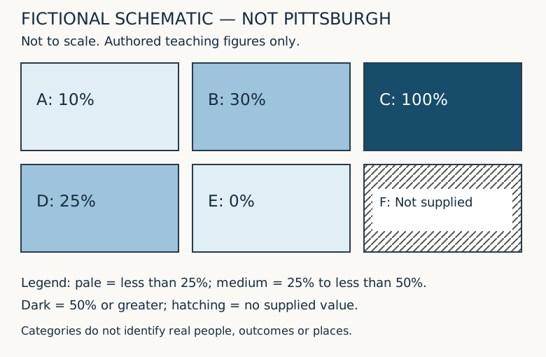
This guide uses an original six-area schematic to practice map reading. Areas A through F are invented rectangles, not Pittsburgh neighborhoods, Census tracts, property parcels or service districts. Every count and percentage is fictional. The schematic is not drawn to geographic scale and cannot be used for navigation or property decisions. Its purpose is to make interpretation choices visible. Use the actual public map and its documentation for a real local question, and keep this teaching exercise separate from claims about residents or places.
Read the map's claim before its visual pattern
Start by looking for the title, publisher, date, geographic coverage and measurement definition. A title such as recorded visits by service area describes something different from residents receiving a service. Visits may include repeat visits by one person, while residents suggests a population definition. A map can be technically well drawn and still answer a different question from the one you intended to ask. Read the full title and explanatory note rather than relying on a social-media caption attached to a cropped image.
For the fictional example, suppose the claim is the share of invented registered records marked complete in six teaching areas during one defined period. That wording is deliberately narrow. It does not claim to measure all residents, all households or the quality of a real service. The denominator is the registered-record count supplied in the worksheet. The word complete refers only to an invented status. A reader should not infer a real program outcome, eligibility decision or level of need from these figures.
Ask whether the publisher supplies enough detail to reconstruct the claim. If a caption says recent data, look for the actual period. If a source note names a dataset, check the version or release and the definition of the field being mapped. If that information is absent, the right conclusion may be that the map cannot answer your question yet. Do not fill missing context with assumptions simply because the visual pattern seems familiar or the map uses an official-looking base layer.
Distinguish points, lines and filled areas
A point symbol often marks a location or an observation, but its precise meaning depends on the legend. In a directory map, it might mark a business address. In another map, a point might stand for multiple records or an approximate location. A line might show a route, boundary or proposed connection. A filled area might summarize a category or quantity within a boundary. Read what each symbol stands for before treating it as a physical feature or a precise measurement.
Imagine an invented point labeled sample meeting location placed inside Area B. Its position would not establish that the whole area is within walking distance, that an entrance is accessible or that a route across the area exists. Similarly, drawing a straight line between two points does not establish a usable path between them. The schematic contains no actual streets, crossings, grades, access permissions or travel times. A real route question requires the relevant current information and, where necessary, direct confirmation.
A filled boundary can also be mistaken for an exact footprint. A service-area polygon may describe administrative coverage, while a shaded statistical area describes the unit used to summarize data. Neither automatically shows a property's legal boundary. If the decision concerns a parcel, zoning designation, district assignment or access right, find the authoritative source for that particular purpose. This guide explains reading habits; it does not validate any map as a survey, legal determination, real-time operational source or proof of permission.
Translate every legend entry into words
The fictional schematic uses three filled categories: less than twenty-five percent, twenty-five percent to less than fifty percent, and fifty percent or greater. A separate hatched symbol means no supplied value. These ranges are invented for the exercise. They are not official thresholds or recommended policy categories. Read the lower and upper limits carefully. A value exactly equal to twenty-five belongs in the second category, while a value exactly equal to fifty belongs in the third under this stated rule.
If a real legend uses ranges such as zero to twenty-five and twenty-five to fifty without explaining endpoints, a boundary value may be ambiguous. Look for the underlying classification definition rather than deciding by color alone. A legend can also use rounded labels while the actual classification operates on more precise values. The displayed label and the classification rule should be consistent enough for the reader to understand. If they are not, preserve the uncertainty in your interpretation rather than claiming a precise category assignment.
Describe a color in terms of its meaning when discussing the map. Instead of saying the blue neighborhood is doing worse, say the map assigns that area to its stated category, then explain the measure and limits. Color is a visual encoding, not an explanation. The category may concern counts, percentages or another measure that does not imply better or worse. Avoid assigning a value judgment to a palette unless the map's documented question actually supports that interpretation.
Work through the six original teaching areas
Area A has ten completed records out of one hundred registered records, so its fictional share is ten percent. Area B has thirty out of one hundred, or thirty percent. Area C has twenty out of twenty, or one hundred percent. Area D has fifty out of two hundred, or twenty-five percent. Area E has zero completed records out of fifty registered records, or zero percent. Area F has no supplied numerator or denominator and therefore no calculated share in the exercise.
Under the invented legend, A and E belong in the less-than-twenty-five category, B and D in the twenty-five-to-less-than-fifty category, and C in the fifty-or-greater category. F receives hatching for no supplied value. These assignments follow the explicit endpoints. Notice that A and E share a category despite having different values, and B and D share another. A categorical map reduces detail. Being the same color does not mean two areas have the same count or percentage.
The accompanying table and CSV preserve the exact teaching inputs. Use them to check the visual classification rather than estimating values from the shade. If a real map has a data table or download, compare its definitions with the displayed map. A mismatch can arise from filters, dates, rounding or an error. Investigate the reason rather than assuming either presentation is automatically correct. A downloadable file is useful evidence of what was supplied, but it still needs a clear source and scope.
Do not confuse a count map with a percentage map
The fictional completed counts are ten in A, thirty in B, twenty in C, fifty in D and zero in E. D has the largest completed count among the supplied areas, yet C has the highest percentage. The difference follows from their denominators: D has two hundred registered records, while C has twenty. A count map and a percentage map could therefore produce different visual rankings without contradicting each other. They are answering different questions using the same invented inputs.
A reader interested in the volume of recorded activity may need counts. A reader interested in the fraction of a defined population may need a percentage or rate. Neither is universally more informative. State the question before choosing the display. In a real local discussion, a high count in a larger population does not automatically show a higher individual likelihood. Conversely, a high percentage in a small denominator does not necessarily mean the largest number of affected people is located there.
The existing percentage-reading guide explores denominators in more detail. The spatial question adds another layer: each denominator belongs to a particular boundary and period. A percentage for a county cannot simply be painted onto a smaller neighborhood because the label is convenient. The map's geographic unit is part of the measurement definition. When repeating a map claim in an article or meeting, carry that unit along with the number rather than replacing it with a more familiar place name.
Keep zero separate from no supplied value
Area E has a defined denominator of fifty and a numerator of zero. Under the teaching definition, its share is zero percent. Area F has no supplied values. It cannot be assigned zero percent merely to fill the empty space. In the schematic, hatching distinguishes F from the pale fill used for low supplied percentages. The difference is important because zero is a value, while the missing entry means this exercise has no basis for calculating a value there.
A real map's blank or gray area could have another documented meaning, such as outside coverage, unavailable data or a suppressed result. Do not assume that every blank is the same kind of missingness. Read the legend and notes for that map. If no explanation is provided, describe the area as not explained by the supplied display rather than asserting that no people, events or services exist there. An absent symbol is not automatically evidence that the underlying activity is absent.
If you make a screenshot for discussion, retain the missing-value symbol in the legend. Cropping it away can turn a cautious display into an apparently complete ranking. The same problem can occur when copying only the colored values into a spreadsheet and omitting unknown rows. Preserve what was excluded and why. Completeness of the picture and completeness of the underlying data are separate questions, and neither should be inferred solely from a map that fills the available screen neatly.
Check the geographic unit and boundary vintage
Census guidance recommends checking geographic boundaries when comparing data over time because the referenced area may have changed. That is a distinct issue from whether a number was calculated correctly. A label or identifier may look familiar while the area it describes differs between releases. Before interpreting a change on two local maps, identify the geography used in each, its boundary vintage and whether the comparison method accounts for any changes. Do not assume that similarly named areas are necessarily identical.
For an original boundary thought experiment, imagine Area A and Area B combined into a single teaching area. Their completed counts add to forty and their registered counts add to two hundred, producing twenty percent. That combined percentage does not mean either original area's percentage changed. It describes a new aggregate. If a later map displays the combined area while an earlier one displays A and B separately, a visual change can reflect the presentation boundary as well as any underlying activity.
Now imagine an old area split into two new areas, but the only available old data are the total for the unsplit area. Do not divide that total equally between the new shapes unless an appropriate method and evidence justify doing so. Equal land area does not establish equal population or equal activity. A real comparison may require relationship files, compatible source data or specialist geographic analysis. The teaching schematic provides no method for estimating actual historical neighborhood statistics across changed boundaries.
Read scale as a relationship, not a travel promise
The USGS publication description explains map scale as the proportion used to represent ground features at a smaller size. In a simplified original arithmetic exercise, a stated scale of one to ten thousand means one unit on the correctly sized map corresponds to ten thousand of the same units in the represented distance. Two centimeters would therefore correspond to twenty thousand centimeters, or two hundred meters, under that simplified relationship. This calculation is separate from the six-area schematic, which has no geographic scale.
Resizing a map can change what a ruler measurement means. If that example map is printed at half its intended linear size, a feature originally spanning two centimeters spans one centimeter on the new print. Applying the original representative fraction to the resized sheet without accounting for the change would misstate the represented distance. A scale bar that resizes with the map may help a reader interpret a copy, but verify that the bar and map were actually resized together rather than pasted separately.
Even a correctly interpreted straight-line distance does not establish travel time or route length. A river, grade, missing connection or access condition may change the practical route. The exercise contains no Pittsburgh travel measurement or accessibility finding. If the real question is whether someone can reach a location by a particular means, use the relevant current route information and confirm material uncertainties. Do not turn a map's geometric proximity into a promise about walking time, driving time or usable access.
Notice how classification changes the picture
The same fictional values can be displayed under another legend without changing the underlying records. Suppose the categories become less than thirty percent, thirty percent to less than sixty percent, and sixty percent or greater. Area D at twenty-five percent moves from the middle category of the first legend to the lower category of the second. Its numerator remains fifty and its denominator remains two hundred. A color change between maps can therefore result from a changed classification rule rather than changed activity.
That does not make either invented classification inherently dishonest. Different categories can serve different explanatory purposes. The reader needs to know the rule and whether it changed. When comparing two real maps, examine both legends rather than assuming that dark blue represents the same interval in each. A publisher might adjust categories to the distribution of each year's values. In that case, similar colors across years may not represent similar numbers, and different colors may not establish a large numerical change.
A table can help test an impression created by the palette. Compare exact values or documented ranges for the areas relevant to your question. Avoid estimating a precise numerical difference from two shades. If the source only supplies categories, preserve that limitation. The fictional example supplies exact values precisely so the reader can see what the category hides. A real map may not provide that level of detail, and a confident visual impression cannot recover data that were not supplied.
Do not infer individual facts from an area summary
Area B's thirty-percent teaching share describes thirty completed records out of one hundred registered records in that invented area. It does not tell you the status of a particular person or address inside the rectangle. A point placed within B does not automatically inherit the area's aggregate result as an individual fact. The area summary can support an appropriately bounded description of the records, but it cannot identify which individual observation has which status without the relevant underlying information.
This matters when a local map is used to describe residents, businesses or properties. A shaded region can be useful for discussing patterns at its documented level, yet it does not establish that every member of the region shares the mapped characteristic. Resist turning a statistical summary into a label for a specific person or location. If a real decision requires individual or property-specific evidence, obtain the appropriate evidence through authorized sources rather than extrapolating from the area color.
The schematic also does not show why the invented shares differ. The figures contain no causal variables, collection history or explanation of the status definition beyond the exercise. A real map pattern can prompt questions, but proximity or similar shading alone does not establish a cause. Separate what the map displays from the hypothesis someone proposes about it. That distinction allows a map to start a useful inquiry without allowing an attractive visual to stand in for supporting evidence.
Keep the map's time and source notes attached
A data period, publication date and display-access date are different pieces of information. A map published this month could display data from an earlier year. An interactive page may show one layer's date alongside a different base map's date. Read which date applies to the measure being discussed. In the teaching example, all values belong to one invented period with no calendar claim. The page's publication date does not turn those figures into current Pittsburgh observations.
When saving a map for a meeting, keep enough information to identify the source and state of the display: title, legend, selected layer, active filters, geography, period and relevant notes. A screenshot may not preserve hidden filter settings or a popup's full definition. If the question depends on them, record the source link and the actual settings separately. Do not treat a screenshot alone as proof that a map is current, complete or suitable for a decision beyond its documented purpose.
If two displays disagree, compare their definitions before choosing the one that supports a preferred conclusion. One could use a different boundary vintage, population, status field or period. Another could include a filter not visible in a cropped image. A genuine discrepancy may also be an error requiring clarification. Describe what can be verified and what remains unresolved. This approach is more useful than announcing a contradiction before determining whether the two maps attempted to represent the same thing.
Explain the map in a bounded paragraph
A careful summary of the original schematic would say that it groups five supplied fictional percentages into three explicitly defined categories and marks one area as having no supplied value. It would identify the numerator and denominator, note that areas are invented and not to scale, and avoid claims about Pittsburgh residents, travel or property. That paragraph is longer than saying the darkest area is best, but it carries the information needed to understand what the picture actually supports.
For a real local map, adapt the questions rather than copying the fictional conclusion. What is mapped? What do its symbols mean? Which geography and period apply? What is missing? Is the legend comparable with the other map? What conclusion is being proposed, and does the display provide the evidence needed for it? A reader can often answer some of these immediately and identify the others as follow-up questions. The result is a clearer interpretation, not a certification of the source.
Frequently asked questions
Is the six-area schematic a map of Pittsburgh?
No. It is an original invented arrangement of rectangles A through F with fictional records. It has no actual coordinates, neighborhood boundaries, travel distances or property information. Its only purpose is to demonstrate how legends, missing values and classification choices affect interpretation.
Does the darkest area always have the largest count?
No. In the fictional percentage display, C is highest at one hundred percent but has twenty completed records. D has fifty completed records and a twenty-five-percent share. Counts and shares use different definitions, so read the mapped measure and denominator before comparing areas.
Should an area with no supplied value be shown as zero?
Not in this exercise. E has a supplied zero numerator and a defined denominator, while F has no supplied numerator or denominator. F is hatched separately. For a real map, use its documented missing-value meaning rather than assuming blank, gray and zero are equivalent.
Can two maps use the same colors but different categories?
Yes. Read each legend's intervals and endpoints. The example shows that twenty-five percent moves categories when the lower boundary of the middle class changes from twenty-five to thirty. The underlying value has not changed merely because its fill category changes.
Does a map's scale establish walking time?
No. A geometric distance is different from a usable route and travel time. Current connections, terrain and access conditions may matter. This teaching page provides no route or accessibility determination. Confirm information appropriate to the actual travel question rather than inferring it from visual proximity.
What should I check before comparing maps from different years?
Check the measured field, numerator and denominator, data period, geographic unit, boundary vintage, filters and legend. Census guidance specifically cautions that geography can change. Explain unresolved differences rather than treating a changed color or familiar place label as proof of a comparable change.
Original fictional schematic and exact values
| Area | Completed records | Registered records | Share |
|---|---|---|---|
| A | 10 | 100 | 10% |
| B | 30 | 100 | 30% |
| C | 20 | 20 | 100% |
| D | 50 | 200 | 25% |
| E | 0 | 50 | 0% |
| F | Not supplied | Not supplied | Not calculated |
Original practice files
Download fictional map-values.csv · Download the original schematic.svg. Neither file contains actual city data or a geographic map.
Primary sources and editorial scope
- USGS Map Scales publication description: proportional representation; full PDF fetch returned403 and was not used for additional claims
- Census Bureau: compare geographic boundaries when comparing data over time
AI-assisted website editorial content. Primary source pages read October 26, 2026. Original arithmetic and categories independently checked. No named professional review, actual Pittsburgh statistics, route finding, property determination or institutional endorsement claimed.